China Products Manufacturers Suppliers

In industrial thermal management, selecting the correct heat exchanger directly impacts process efficiency, operational costs, and maintenance requirements. Among the most widely used designs for liquid-to-liquid or liquid-to-gas heat transfer—plate heat exchangers (PHEs) and spiral heat exchangers (SHEs)—each leverages distinct structural and flow-path designs to address specific application challenges. This analysis systematically compares their core characteristics, performance tradeoffs, and ideal use cases to guide technical decision-making.  

1. Foundational Design & Working Principles  

The fundamental difference between PHEs and SHEs lies in their structure, which dictates fluid flow patterns, heat transfer mechanisms, and operational capabilities.  

1.1 Plate Heat Exchangers (PHEs)  

A PHE consists of a stack of thin, corrugated metal plates (typically 0.5–1.5 mm thick) clamped between two end frames. Each plate features a gasketed perimeter that creates sealed, alternating channels between adjacent plates.  

Working Principle  

– Two process fluids (Hot Fluid [HF] and Cold Fluid [CF]) flow through separate, alternating channels. For example:  

  – HF enters the top of Plate 1, flows through its channel, and exits at the bottom.  

  – CF enters the bottom of Plate 2, flows through its channel (adjacent to Plate 1), and exits at the top.  

– Heat transfers through the thin plate walls, with the corrugated design enhancing fluid turbulence (even at low flow rates) and maximizing the effective heat transfer area.  

Core Structural Features  

– Plates: Materials include 316L stainless steel (standard), titanium (for corrosive fluids like seawater), or Hastelloy (for aggressive chemicals). Corrugation patterns (e.g., herringbone, chevron) are optimized for turbulence and pressure drop.  

– Gaskets: Made of nitrile rubber (standard), EPDM (for high temperatures), or PTFE (for chemical resistance). Gaskets prevent cross-contamination and define fluid flow paths.  

1.2 Spiral Heat Exchangers (SHEs)  

An SHE is constructed by winding two flat metal sheets (typically 1–3 mm thick) around a central cylindrical core, creating two concentric, spiral-shaped channels (one for each fluid). The sheets are separated by spacer studs to maintain channel width, and the edges are welded or gasketed to seal the channels.  

Working Principle  

– Fluids flow in countercurrent (most common) or cocurrent paths through the spiral channels:  

  – HF enters the outer edge of one spiral channel, flows inward toward the core, and exits at the center.  

  – CF enters the center of the second spiral channel, flows outward toward the edge, and exits at the perimeter.  

– The long, narrow spiral path generates high turbulence (even for viscous fluids), while the countercurrent flow maximizes the log mean temperature difference (LMTD)—a key driver of heat transfer efficiency.  

Core Structural Features  

– Metal Sheets: Typically 304/316 stainless steel (standard) or duplex stainless steel (for high pressure/corrosion). Welded construction eliminates gaskets (in most industrial models), reducing leak risk.  

– Channels: Width ranges from 5–25 mm, with larger widths used for fluids with high particulate content (to prevent clogging).  

2. Key Performance & Operational Differences  

The following table compares PHEs and SHEs across critical technical metrics, including heat transfer efficiency, fouling resistance, and maintenance requirements:  

| Metric                  | Plate Heat Exchangers (PHEs)                                                                 | Spiral Heat Exchangers (SHEs)                                                                 |  

|————————-|———————————————————————————————-|———————————————————————————————-|  

| Heat Transfer Efficiency | High (LMTD up to 5–10°C). Corrugated plates create intense turbulence, ideal for low-to-moderate viscosity fluids (≤50 cP). | Very High (LMTD up to 2–5°C). Countercurrent flow + spiral-induced turbulence optimize LMTD, outperforming PHEs for viscous fluids (≥50 cP) or high-temperature applications. |  

| Fouling Resistance  | Low to Moderate. Narrow channels (2–5 mm) and sharp flow turns increase risk of particulate buildup or scaling (e.g., hard water, high-solids fluids). Requires frequent cleaning. | High. Wide, smooth spiral channels (5–25 mm) and continuous flow minimize dead zones. Turbulence creates a “scrubbing effect” that reduces fouling—ideal for fluids with solids (e.g., wastewater, slurries) or scaling potential (e.g., CaCO₃-rich water). |  

| Pressure Drop       | Moderate to High. Turbulence and zigzag flow path increase pressure drop (typically 50–200 kPa). Sensitive to flow rate changes. | Low to Moderate. Smooth spiral flow path reduces pressure drop (typically 20–100 kPa), even for high-viscosity fluids. More stable under variable flow conditions. |  

| Maintenance Access  | Excellent. Plates can be fully disassembled (by removing the end-frame clamp) for inspection, cleaning, or gasket replacement. No specialized tools required. | Limited. Welded construction (no disassembly) means cleaning relies on in-place methods (e.g., CIP—Clean-in-Place, high-pressure water jets). Gasketed SHEs (rare) allow partial disassembly but are less common in industrial use. |  

| Compactness         | Very Compact. High surface area density (200–1,000 m²/m³) — up to 5x more compact than shell-and-tube exchangers, but slightly less so than SHEs for equivalent heat load. | Extremely Compact. Surface area density (300–1,200 m²/m³) — smallest footprint of any heat exchanger type. Ideal for space-constrained installations (e.g., offshore platforms, urban factories). |  

| Fluid Compatibility | Limited by gaskets. Risk of cross-contamination if gaskets degrade. Not suitable for fluids with high particulate content (>50 ppm) or abrasives (e.g., slurries). | Excellent. Welded design eliminates cross-contamination risk. Wide channels handle particulates up to 10 mm (with proper filtration) and abrasive fluids (e.g., mining slurries). |  

| Operating Limits    | Temperature: Up to 200°C (gasket-limited). Pressure: Up to 30 bar (plate/gasket strength-limited). | Temperature: Up to 400°C (weld-limited). Pressure: Up to 100 bar (sheet thickness-limited). Better suited for high-temperature/pressure industrial processes. |  

3. Application Suitability  

The choice between PHEs and SHEs depends on fluid properties, process demands, and operational constraints. Below are their ideal use cases:  

3.1 Plate Heat Exchangers (PHEs)  

Best for applications requiring fast heat transfer, easy maintenance, and clean fluids:  

– HVAC: Chiller systems, heat recovery units (e.g., exchanging heat between fresh air and exhaust air).  

– Food & Beverage: Pasteurization (milk, juice), beer cooling—gasketed design prevents contamination, and easy disassembly meets hygiene standards (e.g., FDA, EU 10/2011).  

– Pharmaceuticals: Drug formulation cooling, clean-in-place (CIP) systems—titanium plates and PTFE gaskets comply with strict purity requirements.  

– Light Industry: Hydraulic oil cooling, low-viscosity chemical processing (e.g., glycol-water mixtures).  

3.2 Spiral Heat Exchangers (SHEs)  

Best for applications with viscous fluids, high fouling potential, or space constraints:  

– Wastewater Treatment: Cooling of sludge or effluent—wide channels resist clogging, and fouling resistance reduces cleaning frequency.  

– Chemical Processing: Handling viscous fluids (e.g., polymers, heavy oils) or high-temperature reactions (e.g., distillation column reboilers).  

– Mining & Minerals: Cooling of abrasive slurries (e.g., ore processing) or scaling fluids (e.g., limewater).  

– Oil & Gas: Offshore platform cooling (compact footprint), crude oil heating, or produced water treatment.  

4. Cost Considerations  

Cost is a critical factor in selection, with tradeoffs between upfront investment and long-term operational expenses:  

| Cost Type               | Plate Heat Exchangers (PHEs)                                                                 | Spiral Heat Exchangers (SHEs)                                                                 |  

|————————-|———————————————————————————————-|———————————————————————————————-|  

| Upfront Cost        | Lower (20–30% less than SHEs for equivalent heat load). Plates and gaskets are mass-produced, reducing manufacturing costs. | Higher. Custom winding and welding (for industrial models) increase production complexity. Gasketed SHEs are cheaper but less durable. |  

| Operational Cost    | Higher. Frequent cleaning (labor, downtime) and gasket replacement (every 1–3 years) add to long-term expenses. | Lower. Reduced cleaning frequency (1–5 years between major maintenance) and no gasket replacement (welded models) minimize operational costs. |  

| Lifespan            | 10–15 years (gasket degradation limits lifespan). Plates can be reused if not corroded.       | 15–25 years (welded construction is corrosion-resistant). Minimal component wear under normal operation. |  

5. Decision Framework: How to Choose  

Use this step-by-step framework to align the exchanger type with your application:  

1. Analyze Fluid Properties:  

   – If fluids are clean, low-viscosity (≤50 cP), and require frequent hygiene checks (e.g., food/pharma): Choose PHE.  

   – If fluids are viscous (≥50 cP), high-fouling, or contain particulates: Choose SHE.  

2. Evaluate Process Conditions:  

   – If operating at low-to-moderate temperature/pressure (≤200°C, ≤30 bar) and need rapid capacity adjustments (add/remove plates): Choose PHE.  

   – If operating at high temperature/pressure (≥200°C, ≥30 bar) or require countercurrent flow for maximum LMTD: Choose SHE.  

3. Assess Space & Maintenance:  

   – If space is limited but maintenance access is critical (e.g., urban HVAC): Choose PHE (compact + easy disassembly).  

   – If space is extremely constrained and maintenance frequency is a priority (e.g., offshore): Choose SHE (smallest footprint + low cleaning needs).  

4. Calculate Total Cost of Ownership (TCO):  

   – For short-term projects (≤10 years) or low fouling: PHEs have lower TCO.  

   – For long-term projects (≥15 years) or high fouling: SHEs offer better cost efficiency.  

In industrial heat transfer systems—from HVAC chillers to petrochemical condensers—low finned tubes are critical components engineered to enhance thermal efficiency without sacrificing compactness. Unlike high-finned tubes (with fin heights >6 mm), low finned tubes feature modest fin protrusions (typically 1–3 mm) that balance surface area expansion with practicality, making them ideal for applications where high airflow resistance or fouling risk limits the use of taller fins. This guide explores their design principles, types, performance benefits, selection criteria, and industry applications to support technical decision-making.  

1. Core Definition & Working Principle  

Low finned tubes are heat exchanger tubes with integrally formed or bonded fins on their outer surface (rarely inner, for specialized fluid-side enhancement). Their design addresses a fundamental challenge in heat transfer: the mismatch between the high thermal conductivity of tube materials (e.g., copper, stainless steel) and the low heat transfer coefficient of the external fluid (often air or low-velocity liquids).  

Key Working Mechanism  

Heat transfer in a low finned tube occurs in three stages:  

1. Fluid-to-Tube Heat Transfer: Heat from the internal fluid (e.g., refrigerant, process oil) transfers through the tube wall via conduction.  

2. Tube-to-Fin Heat Transfer: Heat moves from the tube wall to the fins—critical for integral fins (no thermal resistance at the tube-fin interface) versus bonded fins (minor resistance from adhesives or brazing).  

3. Fin-to-External Fluid Heat Transfer: The fins expand the effective heat transfer area by 2–5x (vs. plain tubes), accelerating convection to the external fluid (e.g., ambient air, cooling water).  

This surface area expansion eliminates the need for larger-diameter plain tubes, enabling more compact heat exchanger designs while maintaining or exceeding thermal performance.  

2. Classification of Low Finned Tubes

Low finned tubes are categorized by their manufacturing method and material composition, each tailored to specific pressure, temperature, and corrosion requirements.  

| Type                  | Manufacturing Process                                                                 | Key Characteristics                                                                 | Ideal Applications                                                                 |  

|———————–|—————————————————————————————|————————————————————————————-|————————————————————————————-|  

| Integral Low Finned Tubes | Fins are extruded, rolled, or forged directly from the tube wall (no separate fin material). | – No tube-fin interface resistance (maximizes thermal efficiency)<br>- High structural integrity (resists fin detachment under pressure/vibration)<br>- Smooth fin roots (minimizes fouling buildup) | High-pressure systems (e.g., refrigerant condensers, hydraulic oil coolers)<br>High-temperature applications (≤400°C for stainless steel) |  

| Seamless Low Finned Tubes | Manufactured from seamless base tubes (via extrusion or piercing) before finning.     | – Eliminates leakage risk at longitudinal seams (critical for toxic/corrosive fluids)<br>- Uniform wall thickness (ensures consistent heat transfer)<br>- Compatible with all finning methods (integral, bonded) | Petrochemical refining (e.g., crude oil coolers)<br>Pharmaceutical processing (sanitary, leak-free requirements) |  

| Bimetallic Low Finned Tubes | Constructed from two metals: a base tube (for structural strength/corrosion resistance) and a fin layer (for high thermal conductivity). | – Optimizes cost-performance (e.g., carbon steel base + copper fins)<br>- Tailored to harsh environments (e.g., duplex stainless steel base + aluminum fins for seawater) | Coastal HVAC systems (corrosion resistance)<br>Industrial heat recovery (high conductivity + low cost) |  

| Bonded Low Finned Tubes   | Fins (typically aluminum/stainless steel strips) are bonded to a plain base tube via brazing, mechanical crimping, or adhesive. | – Lower upfront cost than integral tubes<br>- Flexible material pairing (e.g., copper fins on titanium tubes) | Low-pressure applications (≤10 bar)<br>Low-temperature systems (≤150°C, to avoid adhesive/braze degradation) |  

3. Performance & Operational Benefits  

Low finned tubes outperform plain tubes in key metrics while addressing limitations of high-finned designs. Below are their core advantages:  

3.1 Enhanced Thermal Efficiency  

– Surface Area Expansion: Fins increase the external heat transfer area by 200–500% (e.g., a 25 mm OD plain tube with 2 mm fins achieves ~3x the surface area). This reduces the “thermal resistance bottleneck” of the external fluid, boosting overall heat transfer coefficient (U-value) by 30–60% vs. plain tubes.  

– Reduced Airflow Resistance: Shorter fins (1–3 mm) create less drag for air-side applications (e.g., HVAC coils) than high fins, lowering fan energy consumption by 10–20%.  

3.2 Compact Design  

By maximizing surface area per unit length, low finned tubes allow heat exchangers to achieve the same thermal duty with 40–60% less footprint than plain tube systems. This is critical for space-constrained installations (e.g., rooftop HVAC units, offshore platforms).  

3.3 Cost-Effectiveness  

– Lower Capital Cost: Compact designs reduce the number of tubes, headers, and support structures needed—cutting heat exchanger upfront costs by 15–30%.  

– Reduced Operational Costs: Higher thermal efficiency lowers energy consumption (e.g., smaller fans, pumps), while shorter fins minimize fouling (reducing cleaning frequency and downtime).  

– Longevity: Integral and seamless designs resist corrosion and fin detachment, extending service life to 15–20 years (vs. 8–12 years for bonded high-finned tubes).  

3.4 Versatility  

Low finned tubes adapt to diverse fluids and environments:  

– Fluids: Compatible with refrigerants (R-410A, R-32), process oils, cooling water, and mild chemicals.  

– Environments: Perform reliably in temperatures from -40°C (HVAC refrigeration) to 400°C (petrochemical heating) and resist mild corrosion (with stainless steel or bimetallic construction).  

4. Critical Selection Criteria  

Selecting low finned tubes requires aligning their design with application-specific constraints. Below are the key factors to evaluate:  

4.1 Operating Conditions  

– Temperature Range:  

  – For low temperatures (-40°C to 150°C): Copper or aluminum low finned tubes (excellent thermal conductivity).  

  – For high temperatures (150°C to 400°C): Stainless steel (304/316) or alloy steel tubes (resist thermal fatigue).  

– Pressure Rating:  

  – High-pressure systems (>15 bar): Integral or seamless low finned tubes (structural integrity prevents tube burst).  

  – Low-pressure systems (<10 bar): Bonded tubes (cost-effective).  

4.2 Fluid Properties  

– Internal Fluid:  

  – Corrosive fluids (e.g., acids, seawater): Bimetallic tubes (duplex stainless steel base) or titanium tubes.  

  – Viscous fluids (e.g., heavy oil): Larger fin spacing (3–5 fins per cm) to avoid internal flow restriction.  

– External Fluid:  

  – Air with dust/debris: Low fin height (1–2 mm) + wide fin spacing (reduces fouling).  

  – Cooling water with scaling (e.g., hard water): Integral fins (smooth roots prevent scale buildup).  

4.3 Material Selection  

Choose tube/fin materials based on thermal conductivity, corrosion resistance, and cost:  

| Material       | Thermal Conductivity (W/m·K) | Corrosion Resistance                          | Cost (Relative) | Ideal Environments                                                                 |  

|—————-|——————————-|———————————————–|—————–|————————————————————————————-|  

| Copper         | 401                           | Moderate (resists water, poor for acids)      | Medium          | HVAC refrigeration, potable water cooling                                           |  

| Aluminum       | 237                           | Good (self-healing oxide layer)               | Low             | Low-temperature air cooling (e.g., automotive radiators)                            |  

| 316 Stainless Steel | 16.2                     | Excellent (resists acids, seawater)           | High            | Petrochemical, coastal HVAC, pharmaceutical processing                             |  

| Carbon Steel   | 50.2                          | Poor (requires coating)                       | Very Low        | Low-corrosion industrial heating (e.g., steam condensers with treated water)        |  

4.4 Fin Geometry  

– Fin Height: 1–3 mm (standard); shorter fins (1 mm) for high-airflow applications (e.g., axial fans), taller fins (3 mm) for low-airflow liquids (e.g., cooling water).  

– Fin Spacing: 2–5 fins per cm (fpi: fins per inch). Tighter spacing (5 fpi) for clean air; wider spacing (2 fpi) for dusty or viscous fluids.  

– Fin Thickness: 0.1–0.3 mm (thinner for maximum surface area, thicker for high-vibration applications).  

4.5 Manufacturer Qualification  

– Certifications: Ensure compliance with industry standards (e.g., ASME B31.3 for process piping, ASTM A249 for stainless steel tubes, ISO 9001 for quality management).  

– Track Record: Prioritize manufacturers with experience in your industry (e.g., HVAC-specialized suppliers for chillers, petrochemical-certified suppliers for refineries).  

– Testing Capabilities: Verify the manufacturer conducts thermal performance testing (e.g., U-value measurement) and pressure testing (hydrostatic or pneumatic) to validate tube integrity.  

5. Industry Applications  

Low finned tubes are ubiquitous across sectors where compact, efficient heat transfer is critical:  

– HVAC & Refrigeration: Used in air-cooled condensers (for chillers), evaporator coils (for air handlers), and heat pumps. Their low airflow resistance and compactness make them ideal for rooftop units.  

– Petrochemical & Oil/Gas: Applied in crude oil coolers, refrigerant condensers, and amine gas treating systems. Bimetallic or stainless steel low finned tubes resist corrosive process fluids.  

– Power Generation: Used in transformer oil coolers (air-cooled) and auxiliary cooling systems (for turbines). Seamless designs ensure leak-free operation in high-pressure environments.  

– Food & Beverage: Employed in pasteurizer coolers and beverage chilling systems. Copper or stainless steel tubes meet sanitary standards (e.g., FDA 21 CFR Part 177) and are easy to clean.  

– Automotive & Transportation: Used in engine oil coolers and air conditioning condensers. Aluminum low finned tubes balance lightweight design with thermal efficiency.  

6. Best Practices for Procurement & Maintenance  

6.1 Procurement Tips  

1. Define Performance Metrics: Specify required U-value, pressure rating, and operating temperature range to avoid over- or under-specifying.  

2. Request Samples: Test a small batch for thermal performance (via third-party labs if needed) and corrosion resistance (e.g., salt spray testing for coastal applications).  

3. Negotiate Long-Term Supply: For high-volume applications, secure fixed-price contracts with manufacturers to mitigate material cost fluctuations.  

6.2 Maintenance Guidelines  

1. Regular Inspection: Check for fin damage (bending, detachment) and tube corrosion (via visual checks or ultrasonic testing) quarterly.  

2. Fouling Removal: Clean fins with compressed air (≤6 bar) or low-pressure water jets (for dust/debris). For scaling, use mild chemical cleaners (compatible with tube material) to avoid fin erosion.  

3. Leak Testing: Conduct annual hydrostatic testing (for water-side tubes) or pressure decay testing (for refrigerant tubes) to detect micro-leaks.  

Automatic CNC roll grinders are specialized, high-precision machining systems engineered to maintain and restore the critical surface profiles of rolls used in flat product rolling mills (e.g., steel, aluminum, paper, plastic). These rolls—responsible for shaping, thinning, and finishing flat materials (sheets, coils, films)—require ultra-tight geometric tolerances (±0.001 mm for roundness, ≤0.005 mm/m for straightness) and smooth surface finishes (Ra 0.2–0.8 μm) to ensure consistent product quality. Unlike manual or semi-automatic roll grinders, CNC-equipped models leverage closed-loop control systems, integrated measurement tools, and automated tooling to deliver repeatable results, minimize downtime, and extend roll lifespan. Critical to industries where roll condition directly impacts production efficiency (e.g., a worn roll can cause material defects or line shutdowns), these machines are a cornerstone of modern flat product manufacturing. This article explores their design, operational principles, benefits, applications, and selection criteria—aligned with industry standards (ISO 8688 for grinding processes, API 5L for steel rolling).  

1. Core Role of Rolls in Flat Product Rolling Mills  

To understand the importance of automatic CNC roll grinders, it first helps to contextualize the function of rolls in flat product production:  

– Work Roll: Directly contacts the material (e.g., steel sheet) to reduce thickness and impart surface texture; subject to the highest wear due to friction and pressure (200–500 MPa).  

– Backup Roll: Supports the work roll to prevent deflection (critical for maintaining uniform material thickness across the sheet width).  

– Intermediate Roll: Transfers load between work and backup rolls in multi-stand mills (common in aluminum rolling).  

Over time, rolls degrade due to:  

– Mechanical Wear: Abrasion from the material or contaminants (e.g., scale in steel mills) causes profile distortion (e.g., taper, crown loss).  

– Thermal Fatigue: Cyclic heating/cooling (from friction) leads to surface cracking (“heat checking”).  

– Material Buildup: Adhesion of rolled material (e.g., aluminum oxide) creates “pickup” that damages the product surface.  

Automatic CNC roll grinders rectify these issues by removing a thin layer of material (0.05–0.2 mm) from the roll surface, restoring its original profile, roundness, and finish—ensuring the roll performs optimally until the next maintenance cycle.  

2. Design & Operational Principles of Automatic CNC Roll Grinders  

Automatic CNC roll grinders are distinguished by modular components that enable precision, automation, and adaptability to different roll sizes (length: 1–10 m, diameter: 200–1,200 mm) and profiles (cylindrical, crowned, tapered):  

2.1 Key Components & Their Functions  

| Component               | Design Features                                                                 | Operational Role                                                                 |  

|————————–|———————————————————————————|———————————————————————————–|  

| CNC Control System   | Industrial-grade controller (e.g., Siemens Sinumerik, Fanuc 31i) with roll-specific software; supports 5-axis motion control. | – Executes preprogrammed grinding cycles (e.g., cylindrical grinding, crown grinding). <br> – Integrates real-time feedback from sensors to correct deviations (e.g., roll eccentricity). <br> – Stores 100+ roll profiles for quick changeovers (e.g., switching from steel to aluminum rolls). |  

| Roll Chucking System | Hydraulic or mechanical chucks (3-jaw/4-jaw) with self-centering capability; supports rolls up to 50,000 kg. | – Secures the roll during grinding while minimizing runout (≤0.002 mm). <br> – Adjustable for different roll neck diameters (common in multi-mill operations). |  

| Grinding Wheel Assembly | Large-diameter grinding wheels (600–1,200 mm) with specialized abrasives: <br> – Aluminum oxide (for steel rolls). <br> – CBN (cubic boron nitride) (for hard chrome-plated rolls). <br> – Diamond (for ceramic-coated rolls). | – Removes material via controlled abrasive action; wheel speed (1,500–3,000 RPM) is optimized for roll material. <br> – Automated wheel dressing (via diamond dressers) maintains wheel geometry and sharpness—critical for consistent grinding. |  

| In-Process Measurement System | Laser profilometers or contact probes (e.g., Renishaw) mounted on the grinder carriage. | – Continuously scans the roll surface to verify profile (e.g., crown shape) and dimensions. <br> – Feeds data to the CNC system to adjust grinding parameters (e.g., wheel feed rate) in real time—eliminating the need for manual inspection mid-cycle. |  

| Coolant & Chip Management | High-pressure coolant system (30–50 bar) with directed nozzles; integrated chip conveyors and filters. | – Dissipates heat (prevents thermal distortion of the roll, which can alter profile). <br> – Flushes away abrasive swarf (prevents re-deposition on the roll surface or wheel clogging). <br> – Filters coolant to remove particles (≤10 μm) that cause scratches. |  

2.2 Automated Grinding Process  

The operation of automatic CNC roll grinders is a closed-loop, unattended workflow (typical cycle time: 2–8 hours per roll, depending on size):  

1. Roll Loading: A crane or robotic loader positions the roll onto the grinder’s chucks; the CNC system automatically centers the roll and verifies runout.  

2. Profile Programming: The operator selects a pre-stored roll profile (e.g., “2000 mm steel work roll, 0.05 mm crown”) or inputs custom parameters (e.g., taper for edge thickness control).  

3. Wheel Dressing: The CNC system dresses the grinding wheel to the desired shape (e.g., concave for crown grinding) using a diamond dresser—compensating for wheel wear from previous cycles.  

4. Grinding Execution:  

   – The wheel carriage moves axially along the roll length at a programmable feed rate (0.1–1 mm/rev).  

   – The roll rotates at a synchronized speed (10–50 RPM) to ensure uniform material removal.  

   – In-process sensors monitor the roll’s profile and diameter; if deviations are detected (e.g., 0.003 mm over-tolerance), the CNC adjusts the wheel’s radial feed.  

5. Post-Grinding Inspection: The system performs a final scan to confirm compliance with tolerances; if passing, the roll is unloaded automatically.  

3. Key Benefits of Automatic CNC Roll Grinders  

Compared to manual or semi-automatic alternatives, automatic CNC roll grinders deliver transformative advantages for flat product rolling mills:  

3.1 Enhanced Precision & Product Quality  

– Repeatable Profiles: CNC control eliminates human error (e.g., inconsistent hand feeding), ensuring every roll matches OEM specifications—critical for maintaining uniform material thickness (±0.01 mm across a 2 m wide steel sheet) and surface finish.  

– Minimized Defects: Restoring roll roundness and removing heat checks reduces product defects (e.g., “stripes” from roll eccentricity, “dents” from pickup) by 70–90%, lowering scrap rates (a major cost driver in steel mills).  

3.2 Increased Operational Efficiency  

– Reduced Downtime: Automated loading/unloading and in-process inspection cut grind cycle time by 30–50% vs. manual grinders. For a steel mill running 24/7, this translates to an extra 50–100 rolled tons per day.  

– Lights-Out Operation: CNC systems enable unattended grinding (night/weekend shifts) by auto-adjusting for wheel wear and alerting operators only for critical issues (e.g., coolant low).  

3.3 Extended Roll Lifespan  

– Controlled Material Removal: By removing only the minimum material needed to restore the profile (0.05–0.2 mm per grind), CNC roll grinders extend roll life by 20–30% vs. aggressive manual grinding—reducing roll replacement costs (a single work roll can cost $50,000+).  

– Uniform Wear Management: The system tracks roll usage (e.g., number of grinding cycles) and recommends maintenance before catastrophic failure (e.g., heat check propagation).  

3.4 Cost Savings  

– Labor Reduction: One operator can manage 2–3 CNC roll grinders (vs. 1 operator per manual machine), cutting labor costs by 40–60%.  

– Energy Efficiency: Variable-speed drives and optimized grinding parameters reduce energy consumption by 15–25% vs. older semi-automatic models.  

4. Industry-Specific Applications  

Automatic CNC roll grinders are tailored to the unique demands of flat product rolling mills across sectors:  

4.1 Steel & Aluminum Rolling Mills  

– Application: Grinding work rolls, backup rolls, and intermediate rolls used in hot/cold rolling of flat steel (e.g., automotive sheet, construction plate) or aluminum (e.g., beverage cans, aircraft panels).  

– Critical Requirements:  

  – Ability to grind “crowned” profiles (slight mid-span bulging) to compensate for roll deflection and ensure uniform material thickness.  

  – CBN grinding wheels (for hard chrome-plated rolls) to withstand high wear from steel scale.  

  – Heat-resistant coolant (to handle roll temperatures up to 150°C post-production).  

4.2 Paper & Film Rolling Mills  

– Application: Grinding rolls used in calendering (smoothing paper/film) and casting (extruding plastic films).  

– Critical Requirements:  

  – Ultra-smooth surface finishes (Ra < 0.2 μm) to avoid imprinting defects on paper/film.  

  – Non-marring chucks (to protect soft roll coatings, e.g., rubber in paper calenders).  

  – Precision crown control (to maintain uniform pressure across the roll width—prevents paper “edge curl”).  

4.3 Non-Ferrous Metal Mills (Copper, Brass)  

– Application: Grinding rolls for rolling thin copper sheets (used in electronics, transformers).  

– Critical Requirements:  

  – Low-vibration grinding (to avoid surface chatter on soft copper).  

  – In-process laser measurement (to detect subtle profile deviations that cause electrical conductivity issues in finished copper).  

5. Selection Criteria for Automatic CNC Roll Grinders  

To choose the right machine for a flat product rolling mill, evaluate these technical and operational factors:  

5.1 Roll Compatibility  

– Size Range: Ensure the grinder can accommodate the mill’s largest/smallest rolls (e.g., a 10 m long grinder for steel mill backup rolls vs. a 2 m grinder for plastic film rolls).  

– Weight Capacity: Select a machine with a chuck system rated for the roll weight (e.g., 50,000 kg for heavy steel backup rolls).  

– Profile Capability: Verify support for mill-specific roll profiles (e.g., parabolic crown for aluminum rolling, tapered edges for paper calenders).  

5.2 Precision & Measurement Capabilities  

– Tolerance Range: Choose a grinder with linear scales (0.1 μm resolution) and laser profilometers to meet the mill’s product requirements (e.g., ±0.001 mm for steel automotive sheet rolls).  

– Feedback Speed: Prioritize systems with real-time data processing (≤10 ms latency) to correct deviations mid-grind—critical for high-wear applications (e.g., steel hot rolling).  

5.3 Automation & Integration  

– Loading/Unloading: For high-volume mills, select a machine with robotic roll loaders (reduces manual handling risks and cycle time).  

– Mill Integration: Ensure compatibility with the mill’s MES (Manufacturing Execution System) for data logging (e.g., roll grind history, maintenance schedules) and production tracking.  

5.4 Durability & Maintenance  

– Build Quality: Opt for grinders with heavy-duty cast iron frames (dampen vibration) and sealed spindle bearings (resist coolant contamination—common in steel mills).  

– Service Support: Choose manufacturers with local service centers and spare parts availability (lead time < 48 hours)—critical for minimizing downtime (a grinder outage can stop a rolling mill line).  

5.5 Cost & Total Lifecycle Value  

– Upfront Cost: Automatic CNC roll grinders range from $500,000 to $2 million+—invest in a machine that matches the mill’s production volume (e.g., a high-speed model for a 24/7 steel mill vs. a mid-range model for a small aluminum shop).  

– Operating Costs: Calculate consumable costs (grinding wheels, coolant) and energy use—CBN wheels cost more upfront but last 10–20x longer than aluminum oxide, reducing long-term expenses.  

An ID OD grinding machine (short for Internal Diameter/Outside Diameter Grinding Machine) is a precision machining tool designed to refine the internal (ID) and external (OD) surfaces of cylindrical or conical workpieces. Unlike single-purpose grinders (e.g., dedicated ID grinders), ID OD machines integrate dual capabilities to achieve tight geometric tolerances (typically ±0.0005–0.002 mm) and ultra-smooth surface finishes (Ra 0.1–0.8 μm)—critical for components where dimensional accuracy directly impacts functionality (e.g., bearing races, hydraulic cylinders, aerospace fasteners). These machines leverage specialized spindles, workholding systems, and CNC (Computer Numerical Control) technology to handle diverse materials (metals, ceramics, composites) and complex geometries, making them indispensable in industries like aerospace, automotive, and medical device manufacturing. This article explores their design, operational principles, types, applications, and key advantages—aligned with ISO 8688 (grinding process standards) and ANSI B5.45 (machine tool accuracy).  

1. Core Definitions: ID vs. OD Grinding

The distinction between ID and OD grinding lies in the surface being processed, each requiring unique tooling and machine configurations:  

1.1 ID (Internal Diameter) Grinding  

ID grinding targets the inner surfaces of cylindrical bores, cavities, or holes (e.g., the inner race of a ball bearing, the bore of a hydraulic valve body). Key characteristics:  

– Tooling: Uses small-diameter grinding wheels (5–50 mm) to fit inside narrow bores; wheels are often made of cubic boron nitride (CBN) or diamond for hard materials (e.g., tungsten carbide, tool steel).  

– Challenges: Limited space for wheel rotation requires high spindle speeds (8,000–20,000 RPM) to maintain effective cutting action; heat buildup is a risk (addressed via high-pressure coolant systems).  

– Key Outputs: Achieves precise bore roundness (≤0.001 mm TIR, Total Indicator Reading), straightness (≤0.002 mm/m), and concentricity with the workpiece’s outer surface.  

1.2 OD (Outside Diameter) Grinding  

OD grinding refines the external surfaces of cylindrical or conical workpieces (e.g., the outer race of a bearing, a crankshaft journal, or a precision shaft). Key characteristics:  

– Tooling: Employs larger grinding wheels (200–600 mm diameter) with broader contact areas for efficient material removal; common abrasives include aluminum oxide (for steel) and CBN (for high-hardness alloys).  

– Challenges: Prevents workpiece deflection (critical for long, slender parts) using steady rests or center supports; maintains uniform pressure across the wheel-workpiece interface to avoid taper or out-of-roundness.  

– Key Outputs: Delivers consistent OD diameter, surface finish, and parallelism (for shafts) or taper control (for conical parts like automotive camshafts).  

2. Design & Operational Principles of ID OD Grinding Machines  

ID OD machines combine modular components to handle both internal and external grinding, with precision as the central design priority:  

| Component               | Function (ID Grinding)                                                                 | Function (OD Grinding)                                                                 |  

|————————–|—————————————————————————————–|—————————————————————————————–|  

| Dual Spindles        | – ID Spindle: Small, high-speed (8,000–20,000 RPM) spindle to drive narrow grinding wheels; often uses air bearings for ultra-low vibration. | – OD Spindle: Robust, medium-speed (3,000–6,000 RPM) spindle for large wheels; supports higher grinding forces (5–20 N) for material removal. |  

| Workholding System   | – Collets or Mandrels: Secure the workpiece externally; ensures the bore is concentric with the workpiece’s axis (critical for aerospace components). | – Centers or Chucks: Mount the workpiece between headstock/tailstock centers (for long shafts) or use 3-jaw chucks (for short, heavy parts); steady rests prevent deflection for L/D > 10. |  

| CNC Control System   | – Programs complex ID profiles (e.g., stepped bores, tapers) via 4–5 axis control; integrates in-process probes to measure bore diameter in real time. | – Automates OD grinding cycles (e.g., cylindrical, conical, or crowned profiles); adjusts wheel feed rate to maintain tolerance (±0.0005 mm). |  

| Coolant System       | – Directed nozzles (20–30 bar pressure) deliver coolant to the narrow ID grinding zone; flushes swarf and dissipates heat (prevents thermal distortion). | – Wide-angle nozzles cover the large OD wheel-workpiece interface; coolant filters (≤10 μm) remove particles to avoid scratching. |  

| Wheel Dressing Unit  | – Small diamond dressers (mounted on the spindle) true ID wheels to maintain shape (critical for narrow bores). | – Stationary diamond dressers or rotary dressing tools restore OD wheel geometry and expose fresh abrasive grains. |  

3. Types of ID OD Grinding Machines  

ID OD machines are classified by their automation level and workpiece compatibility, each optimized for specific production needs:  

| Machine Type               | Key Features                                                                 | Ideal Applications                                                                 |  

|—————————–|—————————————————————————–|———————————————————————————–|  

| Manual ID OD Grinder    | – Hand-operated wheel feeds and workpiece positioning; low-cost entry-level option. | Low-volume, simple parts (e.g., small shafts, basic bores) in job shops or repair facilities. |  

| Semi-Automatic ID OD Grinder | – CNC-controlled grinding cycles; manual workpiece loading/unloading.       | Medium-volume production (100–1,000 parts/day) with consistent part geometries (e.g., automotive bearing components). |  

| CNC ID OD Grinder       | – Full 4–5 axis automation; robotic loading/unloading; in-process gauging; MES integration. | High-volume, precision-critical parts (e.g., aerospace turbine shafts, medical implant components); 24/7 lights-out operation. |  

| Universal ID OD Grinder | – Swappable spindles (ID/OD) and workholding (collets/centers); handles cylindrical, conical, and irregularly shaped parts. | Job shops or prototyping labs with diverse part requirements (e.g., grinding a stepped bore one day, a tapered shaft the next). |  

4. Key Applications of ID OD Grinding Machines  

ID OD grinders are integral to industries where dimensional precision and surface quality are non-negotiable. Below are their most critical use cases:  

4.1 Automotive Manufacturing  

– Components: Engine crankshaft journals (OD grinding), hydraulic cylinder bores (ID grinding), transmission gear hubs (both ID/OD for concentricity).  

– Requirements: Tolerances ±0.001–0.003 mm; surface finish Ra 0.2–0.4 μm (to reduce friction in moving parts); concentricity between ID/OD (prevents oil leaks in hydraulic systems).  

4.2 Aerospace & Defense  

– Components: Turbine engine shafts (OD grinding for straightness), aircraft landing gear bushings (ID grinding for bore precision), missile guidance system components (both ID/OD for tight tolerances).  

– Requirements: Ultra-tight tolerances ±0.0005 mm; compatibility with high-temperature alloys (titanium, Inconel); traceability via CNC data logging (for FAA compliance).  

4.3 Medical Device Manufacturing  

– Components: Surgical instrument lumens (ID grinding, e.g., laparoscopic tool channels), orthopedic implant shafts (OD grinding, e.g., hip stem components), dental drill bits (both ID/OD for concentricity).  

– Requirements: Biocompatible materials (stainless steel, titanium); surface finish Ra < 0.1 μm (prevents bacterial adhesion); no micro-cracks (verified via post-grinding NDT, Non-Destructive Testing).  

4.4 Bearing & Hydraulic Industries  

– Components: Ball bearing inner/outer races (ID/OD grinding for roundness), hydraulic valve bores (ID grinding for smooth flow), piston rods (OD grinding for wear resistance).  

– Requirements: Bore roundness ≤0.0008 mm (for bearing performance); OD surface finish Ra 0.1–0.2 μm (reduces seal wear in hydraulic systems); concentricity between ID/OD (≤0.001 mm).  

5. Technical Advantages of ID OD Grinding Machines  

Compared to single-purpose grinders or alternative machining processes (e.g., turning, honing), ID OD machines offer unique benefits:  

5.1 Precision & Consistency  

– Tight Tolerances: Achieve ±0.0005 mm for precision components (e.g., aerospace sensors)—far tighter than turning (±0.005 mm) or honing (±0.001 mm).  

– Repeatability: CNC control eliminates human error, ensuring every part in a batch matches specifications (critical for mass-produced components like bearings).  

5.2 Versatility  

– Material Compatibility: Handle hard metals (tool steel, carbide), soft metals (aluminum, brass), and brittle materials (ceramics, glass) with specialized wheel selection.  

– Geometry Flexibility: Grind cylindrical, conical, stepped, or tapered ID/OD profiles (e.g., a hydraulic valve with a tapered bore and straight OD).  

5.3 Efficiency & Cost Savings  

– Dual Capability: Eliminate the need for two separate machines (ID + OD grinder), reducing floor space (by 30–50%) and capital expenditure.  

– Reduced Secondary Operations: Achieve final surface finish and tolerance in one setup—eliminating post-grinding processes (e.g., polishing) and cutting lead times by 20–40%.  

5.4 Quality & Reliability  

– Heat Control: High-pressure coolant and low-vibration spindles prevent thermal distortion (a major cause of dimensional errors in hard materials).  

– In-Process Inspection: Integrated probes detect deviations mid-grinding and auto-correct parameters—reducing scrap rates to <1% (vs. 5–10% for manual grinding).  

6. Selection Criteria for ID OD Grinding Machines  

To choose the right ID OD grinder, evaluate these critical factors:  

6.1 Workpiece Specifications  

– Size & Geometry:  

  – Small bores (<10 mm diameter) → Require ID spindles with narrow wheels and high RPM (15,000+ RPM).  

  – Long shafts (L/D > 20) → Need OD steady rests to prevent deflection.  

  – Complex profiles (stepped ID/OD) → Require 4–5 axis CNC control.  

– Material Hardness:  

  – HRC > 50 (tungsten carbide, tool steel) → Choose CBN/diamond wheels and rigid machine frames (cast iron with ribbing).  

  – HRC < 30 (aluminum, brass) → Prioritize low-vibration air bearings to avoid surface chatter.  

6.2 Precision & Surface Finish Needs  

– General Manufacturing: ±0.001–0.003 mm tolerance, Ra 0.2–0.8 μm → Semi-automatic CNC machine.  

– Precision Applications: ±0.0005 mm tolerance, Ra < 0.1 μm → Full CNC machine with linear scales (0.1 μm resolution) and in-process laser gauging.  

6.3 Production Volume  

– Low Volume (<100 parts/day): Manual or semi-automatic grinder (lower cost, flexible setup).  

– High Volume (>1,000 parts/day): CNC grinder with robotic loading/unloading and MES integration (24/7 operation).  

6.4 Maintenance & Support  

– Wheel Dressing: Automated dressing units reduce downtime—critical for high-volume runs.  

– Service Availability: Choose manufacturers with local support and spare parts (lead time < 48 hours) to minimize production interruptions.  

In the field of precision machining in modern manufacturing, honed tubes, as core functional components, are driving the high-quality development of over 20 industries such as hydraulic systems and construction machinery with their unique technological advantages. These specially processed steel tubes, finished through honing technology, achieve comprehensive improvement in workpiece performance through precise control of inner hole dimensions, surface quality, and cylindricity.  

I. Core Technological Advantages of Honed Tubes

1. Micron-Level Dimensional Control  

Through the integrated application of CNC honing equipment and real-time detection systems, modern honing processes can precisely control inner diameter tolerance within ±0.005mm (H7-H9 accuracy class), with ovality error not exceeding 0.03mm. This precise dimensional matching extends the service life of equipment seals by 2-3 times, completely solving the leakage problems caused by tolerances in traditional steel tubes.  

2. Super Mirror Finishing Effect  

Using diamond honing sticks combined with intelligent pressure control systems, the inner wall surface roughness can stably reach Ra0.2-0.4μm. The regular oil storage structure formed by special mesh texture processing technology effectively reduces the friction coefficient of moving parts by over 40%.  

3. Enhanced Mechanical Properties  

Through the selection of special steels such as 27SiMn and quenching-tempering processes, the yield strength of honed tubes can reach over 500MPa. Under high-frequency working conditions of 10,000 cycles per minute in heavy machinery, the product maintains stable mechanical performance.  

II. Analysis of Key Application Scenarios  

1. Hydraulic System Innovation  

In the application of hydraulic cylinders for construction machinery, the dimensional stability of high-precision honed tubes enables system pressure to reach 50MPa level. Their ultra-smooth inner walls accelerate hydraulic response speed by 15% and reduce energy loss by 20%, making them the preferred material for hydraulic cylinder manufacturing.  

2. Automotive Manufacturing Upgrade  

After adopting honed tubes for engine cylinder blocks, the inner hole roundness deviation is ≤0.01mm, achieving zero-leakage sealing with piston rings. Test data from an automotive enterprise shows that this technology increases engine power density by 12% and reduces exhaust emissions by 8%.  

3. Intelligent Equipment Transformation  

Miniature honed tubes (outer diameter 17-23mm) used in industrial robot joint parts ensure transmission system positioning accuracy of ±0.005mm through precise dimensional control, meeting the micron-level motion accuracy requirements of intelligent manufacturing equipment.  

III. Advanced Guide to Process Flow  

1. Pretreatment Stage  

Including 11 pre-processing procedures such as raw material screening and precision cold drawing, ensuring the mechanical properties of the base material comply with ISO 9001 standards. Raw material hardness must be controlled within HRC28-32 to lay the foundation for subsequent processing.  

2. Multi-Stage Honing Processing  

Using intelligent honing units for three-step precision grinding: rough honing removes 0.05-0.1mm machining allowance; semi-finish honing improves dimensional accuracy; finish honing achieves nanoscale surface finishing through high-frequency micro-vibration at 6,000 times per minute.  

3. Quality Assurance System  

The entire process is equipped with detection equipment such as laser diameter gauges and 3D profilometers, conducting 100% dimensional inspection of honed tubes. Industry-leading enterprises have established big data traceability systems to ensure process parameters of each product are retrievable.  

IV. Industry Development Trend Forecast  

According to “China Hydraulics and Pneumatics Industry Development Report (2025)”, the global honed tube market size will exceed 8 billion yuan by the end of 2025, with high-precision products (H7 class and above) accounting for 65% of demand. Three major trends—electrification of construction machinery, high-pressureization of hydraulic systems, and miniaturization of precision manufacturing—will drive honing technology toward intelligence and compounding.  

It is recommended that equipment manufacturers, when selecting honed tubes, focus on suppliers’ processing accuracy certification (ISO 2768-mK class), material inspection reports (including metallographic analysis), and practical application cases. For special working condition requirements (such as corrosion resistance and high temperature resistance), customized solutions can be requested from manufacturers.

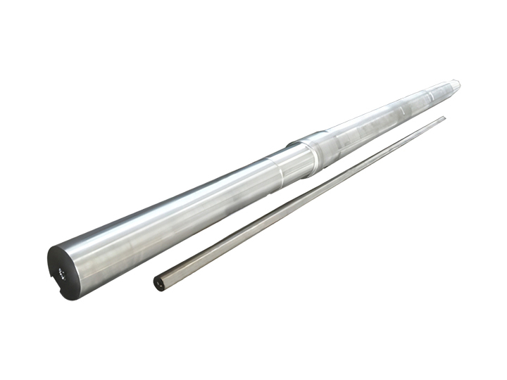
As a core transmission component in the industrial sector, stainless steel shafts occupy a crucial position in mechanical manufacturing due to their unique material advantages. In recent years, demand for stainless steel shafts in China’s industrial market has grown steadily, with products made from 304, 316, and other series accounting for over 65% of the market share. Particularly in the chemical and food processing industries, they have achieved an 8.3% annual compound growth rate, demonstrating strong application potential.  

Core Property Analysis  

1. Exceptional Corrosion Resistance  

In marine environments (salt spray corrosion) and chemical acid-alkaline media, the passive film formed on the surface of stainless steel shafts effectively blocks chemical erosion, with salt spray testing showing no rust for up to 48 hours.  

2. Diversified Strength Adaptation Solutions  

Through heat treatment technologies such as quenching and nitriding, the shaft hardness can be increased to HRC58±2, meeting strength grading requirements from medical devices to heavy-duty equipment.  

3. High-Temperature Operational Stability  

Special stainless steel materials maintain a yield strength >300MPa even at 400°C, suitable for high-load scenarios such as aerospace engines.  

4. Hygienic Safety Design  

Mirror polishing processes with surface roughness Ra≤0.8μm comply with FDA food-grade contact standards, making them core components of dairy filling equipment.  

Industry Application Spectrum  

– Heavy Industry: Stirring shafts for petrochemical reactor kettles are manufactured using duplex stainless steel to withstand hydrogen sulfide corrosion environments.  

– Precision Medical Equipment: Drive shafts for implantable medical devices are ISO13485 certified to ensure biocompatibility.  

– Smart Home Appliances: Rotating shafts in dishwashers utilize 304L ultra-low carbon materials to eliminate intergranular corrosion risks.  

– New Energy Transportation: Drive shafts for electric vehicles adopt lightweight hollow designs, reducing weight by 22%.  

– Special Equipment: Marine platform lifting systems are equipped with 316L material shafting, achieving a 50-year corrosion-resistant design life.  

Advanced Manufacturing Technology Analysis  

1. Material Science Breakthroughs  

New surface composite technologies apply tungsten carbide coatings via laser cladding, tripling wear resistance. A patented technology (CN2022) achieves a shaft scratch resistance rating of 9H pencil hardness.  

2. Precision Forming Processes  

Multi-station cold heading achieves error control within ±0.02mm, and when combined with CNC grinding, key fitting sections maintain roundness errors ≤0.005mm.  

3. Intelligent Quality Monitoring  

Eddy current flaw detectors are integrated for online inspection, identifying internal defects as small as 0.2mm and reducing scrap rates to 0.3‰.  

Usage and Maintenance Guidelines  

– Thermal Expansion Management: Materials with a linear expansion coefficient of 11.5×10⁻⁶/°C require an axial clearance of 0.1mm/m.  

– Welding Process Selection: TIG welding is recommended, with argon purity ≥99.996%.  

– Electrochemical Corrosion Prevention: Avoid direct contact with carbon steel components; insulation bushings are recommended.  

– Lubrication Optimization: For high-temperature conditions, use fully synthetic fluorine grease with a dropping point >280°C.  

As the “power joints” of modern industrial equipment, stainless steel shafts are evolving toward functional complexity and green manufacturing. Third-party testing data shows that process-optimized stainless steel shaft components can extend equipment maintenance cycles by 40%, playing a key role in intelligent manufacturing upgrades. With breakthroughs in surface modification technologies and declining material costs, the penetration rate of these products in new energy vehicle three-electric systems is expected to exceed 35% within five years, creating new market growth drivers.

Nitrogen (N₂) is an inert, colorless, odorless, and tasteless gas—properties that make it indispensable in industrial processes (e.g., inerting, blanketing, purging, cryogenic cooling) but also pose unique detection challenges. Unlike toxic gases (e.g., CO, H₂S), nitrogen’s primary hazard is oxygen displacement: leaks in confined spaces (e.g., tanks, labs, manufacturing cells) reduce ambient oxygen (O₂) levels below the safe threshold (19.5% by volume), leading to rapid asphyxiation—often without warning. Detecting nitrogen leaks promptly requires specialized methods, as the gas itself cannot be directly sensed by human perception or standard toxic gas detectors. This article outlines technical detection methodologies, equipment selection criteria, and best practices for mitigating nitrogen leak risks, aligned with industrial safety standards (e.g., OSHA, NFPA, ISO 23251).  

1. Foundational Context: Why Nitrogen Leaks Are Hard to Detect  

Nitrogen’s physical and chemical properties complicate direct detection:  

– Inertness: It does not react with most materials or generate byproducts (e.g., no corrosive fumes, no exothermic reactions) that could serve as indirect leak indicators.  

– Sensory Transparency: Being colorless, odorless, and tasteless, leaks cannot be identified by sight, smell, or taste—unlike gases such as ammonia (pungent) or chlorine (irritating).  

– Atmospheric Abundance: Since N₂ makes up 78% of ambient air, measuring *absolute nitrogen concentration* is impractical; instead, detection relies on monitoring oxygen depletion (the direct consequence of nitrogen displacement) or using indirect leak-localization techniques.  

The primary risk of undetected leaks is hypoxia:  

– 19.5–23.5% O₂: Normal safe range for human occupancy.  

– 16–19.5% O₂: Mild hypoxia (fatigue, dizziness, impaired judgment).  

– 10–16% O₂: Severe hypoxia (confusion, loss of coordination, unconsciousness).  

– <10% O₂: Fatal within minutes.  

This risk is amplified in enclosed or poorly ventilated spaces (e.g., storage tanks, underground vaults, laboratory fume hoods) where nitrogen can accumulate rapidly.  

2. Technical Detection Methodologies for Nitrogen Leaks

Nitrogen leak detection falls into two categories: oxygen depletion monitoring (to identify hazardous environments) and leak localization techniques (to pinpoint the source of the leak). Below are the most effective, industry-validated methods:  

2.1 Oxygen Depletion Monitoring (Primary Safety Layer)  

Since nitrogen leaks reduce oxygen levels, monitoring ambient O₂ is the most reliable way to detect hazardous nitrogen accumulation. This method does not directly “see” nitrogen but alerts users to the dangerous condition caused by leaks.  

Key Equipment & Operation  

– Fixed Oxygen Monitors: Installed in confined spaces or near nitrogen systems (e.g., piping, tanks). They use electrochemical or optical O₂ sensors to measure real-time O₂ levels and trigger alarms (audible, visual, or remote) when concentrations drop below 19.5% (OSHA’s action threshold).  

  – Electrochemical Sensors: Cost-effective, suitable for normal temperatures (-20°C to 50°C), and require periodic calibration (every 3–6 months).  

  – Optical (Luminance) Sensors: More durable, resistant to poisoning (e.g., from H₂S), and ideal for harsh environments (high humidity, corrosive gases); longer calibration intervals (6–12 months).  

– Portable Oxygen Detectors: Handheld devices for spot checks (e.g., before entering a tank) or mobile monitoring. They typically use electrochemical sensors, have a compact design, and include features like low-battery alerts and data logging.  

Applications  

– Mandatory for confined spaces where nitrogen is used (OSHA 1910.146).  

– Critical for cryogenic nitrogen systems (e.g., liquid nitrogen tanks), where leaks can rapidly vaporize and displace oxygen.  

2.2 Leak Localization Techniques (Secondary: Pinpointing Sources)  

Once an oxygen depletion alarm is triggered, these methods identify the exact leak location (e.g., valve stems, pipe joints, flange gaskets) to enable repairs.  

2.2.1 Ultrasonic Leak Detectors  

– Principle: High-pressure nitrogen leaks generate ultrasonic sound waves (20–100 kHz) as the gas escapes through small orifices—sound frequencies above human hearing range. Ultrasonic detectors amplify these waves and convert them into audible signals or visual readouts.  

– Advantages:  

  – Non-invasive: Detects leaks from a safe distance (1–10 meters), avoiding exposure to hypoxic environments.  

  – Effective in noisy industrial settings: Filters out background noise (e.g., from pumps, motors) using frequency tuning.  

– Limitations:  

  – Ineffective for low-pressure leaks (<1 bar): Insufficient turbulence to generate detectable ultrasonic waves.  

  – Reduced range in open areas: Sound waves dissipate quickly in unconfined spaces.  

– Best For: High-pressure nitrogen systems (e.g., pipelines, pressure vessels), valve packs, and flange connections.  

2.2.2 Infrared (IR) Thermal Imaging Cameras  

– Principle: Nitrogen leaks (especially cryogenic liquid nitrogen, LN₂) cause localized temperature drops: LN₂ vaporizes at -196°C, cooling surrounding surfaces (e.g., pipes, valves) and condensing moisture from the air into frost or fog. IR cameras detect these thermal anomalies (cold spots) and display them as visual images.  

– Advantages:  

  – Rapid area scanning: Covers large surfaces (e.g., entire pipe racks) in minutes, ideal for large-scale facilities.  

  – Non-contact: Eliminates the need to access hard-to-reach areas (e.g., overhead pipes).  

– Limitations:  

  – Ineffective for ambient-temperature nitrogen leaks: No significant thermal contrast with surrounding air.  

  – Requires visible moisture: Works best in humid environments (moisture enhances thermal signature); less effective in dry conditions.  

– Best For: Cryogenic nitrogen systems (e.g., LN₂ storage tanks, transfer lines) and cold nitrogen process equipment.  

2.2.3 Soap Bubble Testing (Manual, Low-Cost)  

– Principle: A soapy water solution (commercially formulated leak-detection soap or a 1:1 mixture of dish soap and water) is applied to potential leak points (e.g., valve threads, gasket seals). Escaping nitrogen gas forms persistent bubbles, indicating the leak source.  

– Advantages:  

  – Low cost: Requires no specialized equipment beyond soap and a brush/spray bottle.  

  – High precision: Pinpoints small leaks (down to 1×10⁻⁶ std cm³/s) in low-pressure systems.  

– Limitations:  

  – Labor-intensive: Requires manual application, making it impractical for large facilities.  

  – Risk of contamination: Soap residue can corrode sensitive components (e.g., electrical connections, precision valves) if not cleaned.  

  – Inaccessible areas: Cannot be used on overhead or enclosed components.  

– Best For: Small-scale systems (e.g., laboratory gas lines, small valves), post-repair verification, or as a supplementary method for confirming leaks detected by ultrasonic/IR tools.  

2.2.4 Tracer Gas Leak Detection (High-Precision, Industrial-Grade)  

– Principle: For critical systems (e.g., semiconductor manufacturing, aerospace), nitrogen is mixed with a small amount of a traceable gas (e.g., helium, hydrogen) that is easy to detect. The system is pressurized, and a handheld tracer gas detector scans for escaping tracer gas—indicating a nitrogen leak.  

– Advantages:  

  – Ultra-high sensitivity: Detects leaks as small as 1×10⁻¹² std cm³/s, suitable for vacuum systems or high-purity applications.  

  – Direct detection: Eliminates reliance on oxygen depletion or thermal cues.  

– Limitations:  

  – High cost: Requires tracer gas and specialized detection equipment.  

  – System downtime: The nitrogen system must be temporarily taken offline to inject tracer gas.  

– Best For: High-purity nitrogen systems (e.g., semiconductor wafer fabrication, pharmaceutical lyophilization) where even micro-leaks are unacceptable.  

3. Equipment Selection Criteria for Nitrogen Leak Detection  

Choosing the right detection tools depends on operational needs, environmental conditions, and risk levels. Key criteria include:  

3.1 Sensitivity & Detection Range  

– Oxygen Monitors: Select devices with a measurement range of 0–25% O₂ and a resolution of 0.1% O₂—critical for detecting gradual oxygen depletion (e.g., a 0.5% drop over 10 minutes).  

– Ultrasonic Detectors: Opt for models with a frequency range of 20–100 kHz and adjustable sensitivity to filter out background noise (e.g., 60 dB in manufacturing plants).  

– IR Cameras: Choose cameras with a thermal sensitivity of <0.1°C (at 30°C) to detect subtle temperature drops from LN₂ leaks.  

3.2 Environmental Compatibility  

– Temperature: For cryogenic applications, select oxygen monitors rated for -40°C to 85°C (to withstand LN₂ vapor exposure). For high-temperature environments (e.g., near furnaces), choose IR cameras with a temperature range of -20°C to 600°C.  

– Humidity/Corrosion: In wet or corrosive areas (e.g., chemical plants), use IP67/IP68-rated equipment (waterproof, dustproof) and optical oxygen sensors (resistant to chemical poisoning).  

– Explosive Environments: In hazardous locations (e.g., refineries), select intrinsically safe (IS) certified detectors (ATEX Zone 0/1, Class I Div 1) to prevent ignition of flammable gases.  

3.3 Usability & Integration  

– User-Friendliness: Prioritize devices with intuitive interfaces (e.g., touchscreens, one-button calibration) and clear alarms (e.g., 90 dB audible alerts, red LED beacons) to ensure quick recognition by untrained personnel.  

– Data Logging & Remote Monitoring: For large facilities, choose fixed oxygen monitors with Modbus/Ethernet connectivity to integrate with SCADA systems—enabling real-time alerts to safety teams and historical data tracking for compliance audits.  

– Portability: For fieldwork or confined space entry, select handheld detectors weighing <500 grams with long battery life (>8 hours of continuous use).  

3.4 Compliance with Standards  

Ensure equipment meets global safety certifications:  

– OSHA 1910.146: Oxygen monitors must trigger alarms at ≤19.5% O₂ (lower explosive limit for oxygen).  

– ISO 23251: For gas detection systems, ensures accuracy and reliability in industrial environments.  

– ATEX/IECEx: For explosive atmospheres, confirms intrinsic safety.  

4. Best Practices for Effective Nitrogen Leak Detection & Mitigation  

Detection equipment alone is insufficient—implement these protocols to minimize risk:  

4.1 Conduct Regular Inspections & Calibration  

– Calibration: Oxygen monitors require monthly “bump tests” (exposure to a known gas concentration to verify alarm functionality) and quarterly full calibrations (using 0% O₂ and 20.9% O₂ standards). Ultrasonic detectors and IR cameras should be calibrated annually by the manufacturer.  

– Pre-Use Checks: Before entering a confined space with nitrogen, use a portable oxygen detector to confirm O₂ levels are ≥19.5%. Inspect hoses, valves, and connections for physical damage (e.g., cracks, loose fittings) that could indicate leaks.  

4.2 Train Personnel on Leak Response  

– Hazard Awareness: Train employees to recognize hypoxia symptoms (dizziness, shortness of breath, confusion) and understand that nitrogen leaks are “silent”—no smell or sight cues.  

– Emergency Protocols: Conduct quarterly drills on:  

  1. Evacuating hypoxic areas immediately (do not attempt to rescue others without self-contained breathing apparatus, SCBA).  

  2. Activating ventilation systems (e.g., exhaust fans, air purifiers) to restore oxygen levels.  

  3. Using leak-localization tools (e.g., ultrasonic detectors) to identify sources after the area is safe.  

4.3 Implement Engineering Controls  

– Ventilation: Install forced-air ventilation in confined spaces (e.g., tanks, labs) to maintain air exchange rates of ≥6 air changes per hour—reducing nitrogen accumulation.  

– Pressure Monitoring: For nitrogen pipelines, install pressure gauges or flow meters; unexpected pressure drops indicate leaks.  

– Secondary Containment: For LN₂ storage tanks, use double-walled vessels with pressure relief valves to contain leaks and prevent rapid vaporization.  

4.4 Document & Review Leak Incidents  

Maintain a leak log to track:  

– Date/time of detection, location, and leak size.  

– Mitigation actions taken (e.g., valve replacement, ventilation activation).  

– Root cause analysis (e.g., worn gaskets, improper installation).  

Review logs quarterly to identify trends (e.g., recurring leaks in a specific pipe section) and implement preventive maintenance (e.g., replacing aging hoses).  

Particulate Matter (PM) sensors—critical for monitoring airborne particle concentrations (e.g., PM₂.₅, PM₁₀) in indoor air quality (IAQ), industrial emissions, and environmental monitoring—rely on unobstructed optical or electrical components to deliver accurate data. Over time, dust, oil, and ambient debris accumulate on sensor surfaces, degrading performance (e.g., skewing light-scattering measurements, blocking airflow). While cleaning is feasible, it requires protocol adherence to avoid damaging sensitive components (e.g., laser diodes, photodetectors). This article details the technical viability of PM sensor cleaning, step-by-step best practices, limitations, and complementary maintenance strategies—aligned with manufacturer guidelines and industry standards (e.g., ISO 16000 for IAQ sensors).  

1. Foundational Context: PM Sensor Design & Why Cleaning Is Necessary  

To understand safe cleaning practices, first contextualize how PM sensors operate—their design dictates which components are vulnerable to fouling and require care:  

Common PM Sensor Technologies & Fouling Vulnerabilities  

Most commercial PM sensors use one of two core technologies, each with distinct high-risk components for contamination:  

| Sensor Technology       | Operating Principle                                                                 | Fouling-Prone Components                                                                 | Impact of Contamination                                                                 |  

|————————-|————————————————————————————–|——————————————————————————————|——————————————————————————————|  

| Optical (Light-Scattering) | A laser or LED emits light into a sampling chamber; particles scatter light, which is detected by a photodetector. Concentration is calculated from scatter intensity. | – Laser/LED emitter lens <br> – Photodetector lens <br> – Sampling chamber walls <br> – Air inlet/outlet filters | – Scratched or dirty lenses reduce light intensity, leading to underestimation of PM concentrations (e.g., a 10% lens occlusion can lower readings by 15–20%). <br> – Clogged inlets restrict airflow, reducing sample volume and accuracy. |  

| Electrical (Gravimetric/Impedance) | Particles accumulate on a weighted filter (gravimetric) or conductive surface (impedance); mass/conductivity changes indicate PM concentration. | – Filter media (gravimetric) <br> – Conductive sensing electrodes (impedance) <br> – Airflow fans/pumps | – Filter clogging halts measurements (gravimetric) or increases pressure drop (skewing airflow). <br> – Oil/dust on electrodes disrupts impedance readings, causing false high/low values. |  

Key Takeaway  

Fouling is not just a performance issue—it can render sensors non-functional. For example, in industrial emissions monitoring, a dirty PM sensor may fail to detect exceedances of regulatory limits (e.g., EPA 40 CFR Part 60), leading to non-compliance fines. Regular cleaning mitigates this risk—*but only if done correctly*.  

2. Is Cleaning a PM Sensor Feasible? Technical Considerations  

The short answer: Yes, but feasibility depends on sensor type (field-serviceable vs. sealed) and component accessibility.  

Critical Distinction: Field-Serviceable vs. Sealed Sensors  

Manufacturers design PM sensors with varying levels of user-accessibility, which dictates whether cleaning is practical:  

– Field-Serviceable Sensors: These have removable covers, accessible lenses, or replaceable filters (e.g., industrial-grade sensors like the TSI DustTrak™, or consumer IAQ sensors like the Awair Element). Cleaning is explicitly recommended by manufacturers for these models.  

– Sealed (Non-Serviceable) Sensors: Miniaturized or low-cost sensors (e.g., some automotive PM sensors, compact IoT sensors) are hermetically sealed to prevent tampering. Opening these voids warranties and often damages internal components (e.g., delicate laser alignment). For sealed sensors, cleaning is not feasible—replacement is the only option if fouling occurs.  

Manufacturer Guidelines: The First Rule of Cleaning  

Always consult the sensor’s user manual before cleaning. Manufacturers provide model-specific instructions (e.g., allowed cleaning agents, disassembly limits) to avoid damage. For example:  

– Some optical sensors prohibit alcohol on emitter lenses (it can dissolve anti-reflective coatings).  

– Gravimetric sensors may require filter replacement (not cleaning) to maintain accuracy.  

Ignoring these guidelines can lead to permanent sensor failure or invalidated calibration certifications.  

3. Step-by-Step Technical Cleaning Protocol (For Field-Serviceable Sensors)  

For accessible PM sensors, follow this industry-standard workflow to minimize risk and maximize effectiveness. The protocol varies slightly by sensor technology but shares core principles of gentleness and precision.  

3.1 Pre-Cleaning Preparation  

1. Safety First:  

   – Power off the sensor and disconnect it from all power sources (AC adapters, USB cables) to avoid electrical shock or short-circuiting components (e.g., fans, circuit boards).  

   – Wear nitrile gloves to prevent oil from your skin transferring to sensor surfaces (skin oil is a common cause of lens fouling and is difficult to remove).  

2. Gather Tools:  

   Use only manufacturer-approved or industry-recommended tools to avoid scratches or chemical damage:  

   – Compressed Air: Ultra-low-pressure (20–30 PSI) canned air with a narrow nozzle (to target specific components); avoid high-pressure air (it can dislodge delicate parts like photodetectors).  

   – Cleaning Agents: Isopropyl alcohol (IPA) (70–99% purity—higher purity reduces residue), or manufacturer-specified lens cleaner (avoid water, ammonia, or abrasive solvents).  

   – Applicators: Lint-free microfiber cloths (for lenses), wooden or plastic toothpicks (for clearing clogged inlets—*never metal*, which scratches plastic), and foam swabs (for sampling chamber walls).  

   – Disassembly Tools: Small Phillips-head or Torx screwdrivers (if the sensor requires opening); use magnetized tools to avoid losing tiny screws.  

3.2 Cleaning Optical PM Sensors (Light-Scattering Type)  

Optical sensors are the most common and require the most care—their lenses and laser components are highly sensitive.  

1. Disassemble (If Required):  

   – Remove the sensor’s outer cover using the appropriate screwdriver. Avoid forcing parts—if something sticks, refer to the manual (some covers use snap-fit designs, not screws).  

   – Locate the sampling chamber (where air and particles interact with light) and identify the emitter lens (near the laser/LED) and photodetector lens (opposite or at a 90° angle to the emitter).  

2. Remove Loose Debris with Compressed Air:  

   – Hold the canned air can 6–8 inches away from the sensor (to reduce pressure) and blow gently across:  

     – The air inlet/outlet grilles (to clear clogged dust).  

     – The sampling chamber walls (to dislodge loose particles).  

     – The edges of the emitter/photodetector lenses (avoid blowing directly onto lens centers—this can push debris into coatings).  

3. Clean Lenses (Delicate Step):  

   – For minor fouling: Lightly dampen a microfiber cloth with 99% IPA (less residue than 70%) and wipe the lens in gentle circular motions (start at the center, move outward). Never scrub—this scratches anti-reflective coatings.  

   – For stubborn residue (e.g., oil): Use a foam swab (not cotton—cotton leaves lint) dipped in IPA, and gently dab the lens (avoid rubbing). Allow the lens to air-dry completely (1–2 minutes) before reassembly—IPA evaporates quickly and leaves no residue.  

4. Reassemble & Test:  

   – Replace the outer cover and secure screws to the manufacturer’s torque specifications (over-tightening can crack plastic housings).  

   – Power on the sensor and run a zero-calibration check (most sensors have a built-in function) to verify accuracy. Compare readings to a calibrated reference sensor (if available) to ensure no post-cleaning drift.  

3.3 Cleaning Electrical PM Sensors (Gravimetric/Impedance Type)  

Electrical sensors focus on filter or electrode maintenance rather than lens care:  

1. Gravimetric Sensors:  

   – These use a disposable filter to collect particles. Do not clean the filter—it is designed for one-time use. Instead, replace the filter per the manufacturer’s schedule (e.g., every 7–30 days for high-PM environments).  

   – Clean the filter housing with compressed air to remove loose dust that could contaminate the new filter.  

2. Impedance Sensors:  

   – Locate the conductive sensing electrodes (usually two metal plates inside the sampling chamber).  

   – Use a dry foam swab to gently brush away loose dust from the electrodes (avoid IPA—some electrodes have conductive coatings that alcohol can dissolve).  

   – For oil residue: Use a swab dampened with deionized water (not IPA) to dab the electrodes, then air-dry completely (water evaporates without damaging coatings).  

4. Critical Limitations & Risks of Cleaning  

While cleaning improves performance, it is not without risks—avoid these common mistakes to prevent sensor damage:  

4.1Insurmountable cleaning restrictions  

– Sealed Sensors: As noted earlier, opening sealed sensors (e.g., some automotive PM₂.₅ sensors) voids warranties and often misaligns internal components (e.g., laser-to-photodetector alignment), rendering the sensor inaccurate.  

– Damaged Coatings: Anti-reflective coatings on optical lenses are fragile—even mild scrubbing or harsh solvents (e.g., acetone) can remove them, permanently reducing light transmission.  

– Calibration Drift: Disassembling and reassembling sensors can shift components (e.g., the sampling chamber) out of alignment. Always perform a post-cleaning calibration (using manufacturer-approved standards) to correct drift.  

4.2 High-Risk Practices to Avoid  

| Risky Practice               | Consequence                                                                 |  

|——————————|——————————————————————————|  

| Using cotton swabs/linty cloths | Lint fibers stick to lenses/electrodes, causing new fouling and inaccurate readings. |  

| High-pressure air (>50 PSI)   | Dislodges delicate parts (e.g., fan blades, photodetector wiring) or bends sensor housings. |  

| Water or aqueous cleaners (on optical sensors) | Water leaves mineral deposits on lenses and can short-circuit circuit boards. |  

| Cleaning hot sensors          | Thermal expansion/contraction during cleaning can crack plastic components or damage solder joints. |  

5. Complementary Maintenance: Beyond Cleaning  

Cleaning alone is not enough to ensure long-term PM sensor accuracy. Pair cleaning with these industry-best maintenance practices:  

5.1 Regular Calibration  

– Calibrate sensors per manufacturer guidelines (e.g., every 3–6 months for industrial sensors, annually for IAQ sensors) using NIST-traceable PM standards (e.g., Arizona test dust for PM₁₀). Calibration corrects for any drift caused by cleaning or component wear.  

– For critical applications (e.g., industrial emissions monitoring), use a reference sensor (e.g., TSI 3016, a EPA-approved gravimetric sensor) to validate readings monthly.  

5.2 Environmental Controls  

– Reduce fouling at the source: Install the sensor away from high-PM or oil-rich environments (e.g., near vents, printers, or industrial ovens) if possible.  

– Use pre-filters: Many sensors accept optional inlet pre-filters (e.g., HEPA pre-filters for IAQ sensors) that capture large particles before they reach the sensor—extending cleaning intervals by 2–3x.  

5.3 Performance Monitoring  

– Log sensor data over time to identify fouling trends (e.g., a gradual drop in PM readings for a known high-PM environment indicates fouling).  

– Set up alerts (via sensor software) for low airflow or reading drift—these are early signs that cleaning is needed.  

6. Self-Cleaning PM Sensors: A Low-Maintenance Alternative  

For high-PM or hard-to-access environments (e.g., industrial chimneys, outdoor air quality stations), self-cleaning PM sensors are a technical solution that reduces manual cleaning needs. These sensors integrate automated cleaning mechanisms:  

| Self-Cleaning Mechanism       | How It Works                                                                 | Advantage                                                                 |  

|——————————–|——————————————————————————|—————————————————————————-|  

| Ultrasonic Cleaning        | High-frequency sound waves vibrate the sensor lens, dislodging dust and debris. | No physical contact—avoids lens damage; works continuously during operation. |  

| Compressed Air Jets (Automated) | A built-in low-pressure air pump periodically blows air across lenses/electrodes. | Reduces manual cleaning intervals from monthly to quarterly. |  

| Heated Sensors             | The sampling chamber is heated to 50–60°C, preventing oil condensation (a common fouling source) on components. | Ideal for high-humidity or oil-rich environments (e.g., kitchens, industrial workshops). |  

Self-cleaning sensors are more expensive upfront but lower lifecycle costs by reducing maintenance labor and sensor replacement frequency.  

A distillation tower (also called a distillation column or fractionating column) is a vertical, industrial-scale separation device designed to fractionate liquid or vapor mixtures into their individual components based on differences in volatility (a property inversely related to boiling point: more volatile components have lower boiling points and vaporize more easily). Critical in petrochemical, oil refining, and chemical manufacturing, these towers enable the production of fuels (gasoline, diesel), solvents (ethanol, methanol), and high-purity chemicals by leveraging the principle of vapor-liquid equilibrium (VLE)—the dynamic balance where vapor and liquid phases coexist, with more volatile components concentrated in the vapor and less volatile components in the liquid. This article breaks down the tower’s design, operational principles, key components, and industrial applications—aligned with chemical engineering standards (e.g., ASTM D2892 for crude oil distillation, ISO 6570 for packed column performance).  

1. Foundational Principle: Vapor-Liquid Equilibrium (VLE)  

Distillation towers rely on VLE to drive separation. When a liquid mixture is heated, its more volatile components (lower boiling points) vaporize first. As this vapor rises and contacts a cooler liquid stream (reflux, explained later), it condenses—transferring heat and mass to the liquid. This interaction enriches the vapor with volatile components and the liquid with less volatile components. Repeating this cycle across multiple “stages” (trays or packing) in the tower achieves progressive separation, producing highly purified fractions.  

For example, in crude oil distillation:  

– Light hydrocarbons (e.g., propane, boiling point -42°C) are most volatile—they rise to the tower’s top.  

– Heavy hydrocarbons (e.g., asphalt, boiling point >500°C) are least volatile—they remain at the tower’s bottom.  

– Intermediate fractions (gasoline, diesel) collect at mid-tower levels, corresponding to their boiling points.  

2. Key Components of a Distillation Tower

A distillation tower’s design is modular, with components working in tandem to optimize vapor-liquid contact and separation efficiency:  

| Component               | Location                          | Function                                                                 | Design Variations                                                                 |  

|————————–|———————————–|————————————————————————–|———————————————————————————–|  

| Column Shell         | Entire structure                  | Vertical, cylindrical vessel (5–100 m tall, 1–10 m diameter) that houses internal components; constructed from corrosion-resistant steel (e.g., 316 stainless steel for chemical service). | – Atmospheric columns (operate at ambient pressure, for crude oil). <br> – Vacuum columns (operate at sub-atmospheric pressure, to separate high-boiling components without thermal degradation). |  

| Internals: Trays or Packing | Inside the column (stacked vertically) | Provide a large surface area for vapor-liquid contact—critical for mass/heat transfer. | – Trays: Horizontal plates with perforations (sieve trays), valves (valve trays), or bubble caps (bubble-cap trays). Vapor rises through holes, bubbles through liquid on the tray, and exits to the next tray; liquid overflows via downcomers to the tray below. <br> – Packing: Loose or structured materials (e.g., Raschig rings, Pall rings, metal sheets) that create a tortuous path for vapor/liquid. Liquid flows downward over packing surfaces; vapor rises upward, interacting with the liquid film. |  

| Reboiler             | Bottom of the column              | Heats the liquid “bottoms” (least volatile fraction) to generate vapor, which rises up the column to initiate separation. | – Kettle reboiler: Heats liquid in a separate vessel, with vapor returning to the column. <br> – Thermosiphon reboiler: Uses natural convection (heated liquid rises, cooled liquid falls) for continuous circulation—common in oil refineries. |  

| Condenser            | Top of the column                 | Cools the overhead vapor (most volatile fraction) into a liquid “distillate.” | – Total condenser: Condenses all vapor into liquid (used for producing liquid products like ethanol). <br> – Partial condenser: Condenses only a portion of vapor; uncondensed vapor (e.g., natural gas) is collected separately. |  

| Reflux System        | Between condenser and column top  | Returns a portion of the condensed distillate (called “reflux”) back to the column’s top tray/packing. Reflux provides the cool liquid needed for vapor-liquid contact, improving separation efficiency. | – Reflux drum: Stores condensed distillate; a pump controls reflux flow rate (typically 1–10x the product withdrawal rate). <br> – Reflux ratio: Ratio of reflux flow to product flow (higher ratios = better separation but higher energy use). |  

| Feed Inlet           | Mid-column (varies by mixture)    | Introduces the raw mixture (“feed”) into the column at a height matching the feed’s volatility profile (called the “feed tray”). This minimizes energy waste by aligning the feed with the column’s internal concentration gradient. | – Subcooled liquid feed: Feed is cooler than the column’s temperature at the feed tray—adds liquid to the column. <br> – Superheated vapor feed: Feed is hotter than the column’s temperature—adds vapor to the column. |  

| Product Outlets      | Top, middle, and bottom           | Extract purified fractions at different heights: <br> – Top outlet: Most volatile fraction (e.g., gasoline in crude distillation). <br> – Side draws (middle): Intermediate fractions (e.g., diesel, kerosene). <br> – Bottom outlet: Least volatile fraction (e.g., heavy fuel oil, asphalt). | – Valves or pumps regulate flow rates; on-line analyzers (e.g., gas chromatographs) monitor purity in real time. |  

3. Step-by-Step Operation of a Distillation Tower  

The tower’s operation follows a continuous, closed-loop process optimized for steady-state separation. Below is a detailed breakdown using crude oil distillation as an example:  

Step 1: Feed Preparation & Introduction  

– The raw mixture (e.g., crude oil) is preheated (to 250–350°C) and pumped into the column via the feed inlet—typically at the mid-column “feed tray.” This preheating reduces the reboiler’s energy load and ensures the feed matches the column’s temperature at that height.  

Step 2: Vapor Generation (Reboiler)  

– At the column’s bottom, the reboiler heats the liquid bottoms (heavy crude components) to 350–400°C. This generates vapor rich in intermediate and light hydrocarbons, which rises upward through the column’s trays or packing.  

Step 3: Vapor-Liquid Contact (Separation Stages)  

– As vapor rises, it interacts with liquid flowing downward (from the reflux system or higher trays):  

  – On Trays: Vapor bubbles through the liquid layer on each tray, transferring heat (vapor condenses, liquid vaporizes) and mass (volatile components move to vapor, less volatile components move to liquid). Liquid overflows via downcomers to the next lower tray, becoming progressively richer in heavy components.  

  – In Packing: Liquid flows downward as a thin film over packing surfaces; vapor rises through the packing’s gaps, contacting the film. This continuous interaction achieves the same separation as trays but with lower pressure drop (ideal for vacuum columns).  

Step 4: Overhead Vapor Condensation  

– Vapor reaching the column’s top (rich in light hydrocarbons like gasoline) flows to the condenser, where it is cooled to 40–60°C (using cooling water or air). This condenses the vapor into liquid distillate, which collects in a reflux drum.  

Step 5: Reflux & Product Withdrawal  

– A portion of the distillate is pumped back to the column’s top as reflux (reflux ratio = 3–5 for crude oil). This reflux provides the cool liquid needed to “scrub” rising vapor, removing heavy contaminants and improving light fraction purity.  

– The remaining distillate is withdrawn as the top product (e.g., gasoline). Intermediate products (e.g., diesel, kerosene) are extracted via side draws at mid-column heights, where their concentration is highest.  

– The least volatile components (heavy fuel oil, asphalt) remain as liquid bottoms, which are withdrawn from the column’s base and sent to downstream processes (e.g., cracking units for further refinement).  

Step 6: Process Control  

– Sensors and controllers maintain steady-state operation:  

  – Temperature sensors: Monitor tray temperatures to adjust reboiler heat (higher temperature = more vapor generation).  

  – Pressure sensors: Regulate column pressure (critical for vacuum columns, where pressure affects boiling points).  

  – Flow meters: Adjust reflux rate and product withdrawal to maintain desired purity (e.g., 95% ethanol in solvent production).  

4. Types of Distillation Towers  

Towers are classified by their internal design (tray vs. packing) and operating pressure, each suited to specific applications:  

| Tower Type               | Key Design Feature                                                                 | Ideal Applications                                                                 |  

|—————————|———————————————————————————–|———————————————————————————–|  

| Tray Column           | Uses perforated, valve, or bubble-cap trays; easy to maintain and scale.          | High-volume, robust separations (e.g., crude oil distillation, petrochemical production) where fouling (solid buildup) is a risk. |  

| Packed Column         | Uses structured/loose packing; lower pressure drop, higher efficiency for small-diameter columns. | Low-pressure or vacuum separations (e.g., separating high-boiling hydrocarbons to avoid thermal degradation), and fine chemical separations (e.g., pharmaceutical solvent purification). |  

| Atmospheric Column    | Operates at ambient pressure (1 atm); no vacuum system needed.                    | Separating low-to-medium boiling mixtures (e.g., crude oil into gasoline, diesel). |  

| Vacuum Column         | Operates at sub-atmospheric pressure (0.01–0.1 atm); reduces boiling points of heavy components. | Separating high-boiling fractions (e.g., crude oil bottoms into lubricating oil, asphalt) without thermal cracking. |  

5. Industrial Applications  

Distillation towers are ubiquitous in process industries, enabling the production of essential materials:  

5.1 Oil Refining  

– Primary Use: Fractionate crude oil into marketable fuels and feedstocks.  

– Products:  

  – Top: Liquefied Petroleum Gas (LPG, propane/butane).  

  – Mid: Gasoline (C5–C12), kerosene (C12–C15), diesel (C15–C20).  

  – Bottom: Heavy fuel oil, asphalt, and feedstocks for catalytic cracking (to make more gasoline).  

5.2 Chemical Manufacturing  

– Primary Use: Purify solvents, monomers, and intermediates.  

– Examples:  

  – Ethanol purification (removing water to 99.5% “absolute ethanol” for pharmaceuticals).  

  – Separation of ethylene/propylene (monomers for plastics) from naphtha crackers.  

5.3 Petrochemicals  

– Primary Use: Produce high-purity hydrocarbons for polymers and specialty chemicals.  

– Example: Separating benzene, toluene, and xylene (BTX) from reformate (a crude oil derivative) for plastic and dye production.  

5.4 Cryogenic Distillation  

– Primary Use: Separate air into oxygen, nitrogen, and argon (requires ultra-low temperatures: -183°C for oxygen, -196°C for nitrogen).  

– Applications: Steel manufacturing (oxygen for combustion), food packaging (nitrogen for inert atmosphere), and electronics (argon for welding).  

6. Challenges & Optimization  

While distillation towers are highly effective, they face key challenges that drive ongoing optimization:  

6.1 Energy Intensity  

– Distillation accounts for ~40% of energy use in chemical plants (due to reboiler heating and condenser cooling).  

– Optimizations:  

  – Heat integration (using waste heat from other processes to preheat the feed).  

  – Variable reflux ratios (lower ratios for less strict purity requirements).  

  – Advanced controls (AI-based systems to adjust pressure/temperature in real time).  

6.2 Fouling & Maintenance  

– Trays or packing can foul with solids (e.g., coke in crude oil columns), reducing efficiency.  

– Solutions:  

  – Periodic cleaning (chemical or mechanical).  

  – Use of fouling-resistant materials (e.g., Hastelloy for corrosive feeds).  

6.3 Environmental Impact  

– Volatile organic compound (VOC) emissions from column vents are a concern.  

– Mitigations:  

  – Closed-loop condensers to capture emissions.  

  – Carbon capture systems (for large-scale towers).